After we fit a model, the effects of covariate interactions are of special interest. With margins and factor-variable notation, I can easily estimate, graph, and interpret effects for models with interactions. This is true for linear models and for nonlinear models such as probit, logistic, and Poisson. Below, I illustrate how this works.
Suppose I want to fit a model that includes the interactions between continuous variables, between discrete variables, or between a combination of the two. I do not need to create dummy variables, interaction terms, or polynomials. I just use factor-variable notation.
If I want to include the square of a continuous variable x in my model, I type
c.x#c.x
If I want a third-order polynomial, I type
c.x#c.x#c.x
If I want to use a discrete variable a with five levels, I do not need to create a dummy variable for four categories. I simply type
i.a
If I want to include x, a, and their interaction in my model, I type
c.x##i.a
Stata now understands which variables in my model are continuous and which variables are discrete. This matters when I am computing effects. If I am interested in marginal effects for a continuous variable on an outcome of interest, the answer is a derivative. If I am interested in the effect for a discrete variable on an outcome, the answer is a discrete change relative to a base level. After fitting a model with discrete variables and interactions specified in this way with margins, I automatically get the effects I want.
Suppose I am interested in modeling the probability of an individual being married as a function of years of schooling (“education”), the percentile of income distribution to which that individual belongs (“percentile”), the number of times he or she has been divorced (“divorces”), and whether his or her parents are divorced (“pdivorced”).
I want to use probit to estimate the parameters of the relationship
$P(y|x, d) = \Phi \left(\beta_0 + \beta_1x + \beta_3d + \beta_4xd + \beta_2x^2 \right)$
I fit the model like this:
. probit married c.education##c.percentile c.education#i.divorces i.pdivorced##i.divorces
Factor-variable notation helps me introduce the continuous variables education and percentile; the discrete variables divorces and pdivorced; and the interactions between education and percentile, education and divorces, and divorces and pdivorced. Stata reports
Probit regression                               Number of obs     =      5,000
                                                LR chi2(10)       =     426.50
                                                Prob > chi2       =     0.0000
Log likelihood = -3001.1256                     Pseudo R2         =     0.0663

------------------------------------------------------------------------------
     married |      Coef.   Std. Err.      z    P>|z|     [95% Conf. Interval]
-------------+----------------------------------------------------------------
   education |   .0023907    .010848     0.22   0.826     -.018871    .0236525
  percentile |     .00675   .6963511     0.01   0.992    -1.358073    1.371573
             |
 c.education#|
c.percentile |   .3615247   .0741706     4.87   0.000      .216153    .5068965
             |
    divorces#|
 c.education |
          1  |   .0372029   .0171671     2.17   0.030     .0035561    .0708497
          2  |   .2162807   .0934079     2.32   0.021     .0332047    .3993568
             |
 1.pdivorced |   -.136213   .0434619    -3.13   0.002    -.2213968   -.0510292
             |
    divorces |
          1  |  -.3059462   .1791099    -1.71   0.088    -.6569953    .0451028
          2  |  -1.930222   .9246691    -2.09   0.037     -3.74254   -.1179043
             |
   pdivorced#|
    divorces |
        1 1  |  -.3123379   .0982202    -3.18   0.001    -.5048458   -.1198299
        1 2  |  -1.033269   .4108841    -2.51   0.012    -1.838587   -.2279512
             |
       _cons |   .1366351   .1092899     1.25   0.211    -.0775692    .3508393
------------------------------------------------------------------------------
Using the results from my probit model, I can estimate the average change in the probability of being married as the interacted variables divorces and education both change. To get the effect I want, I type
. margins divorces, dydx(education) pwcompare
The dydx(education) option computes the average marginal effect of education on the probability of divorce, while the divorces statement after margins paired with the pwcompare option computes the discrete differences between the levels of divorce. Stata reports
Pairwise comparisons of average marginal effects
Model VCE    : OIM

Expression   : Pr(married), predict()
dy/dx w.r.t. : education

--------------------------------------------------------------
             |   Contrast Delta-method         Unadjusted
             |      dy/dx   Std. Err.     [95% Conf. Interval]
-------------+------------------------------------------------
education    |
    divorces |
     1 vs 0  |   .0136111   .0057912      .0022607    .0249616
     2 vs 0  |   .0601653    .019514      .0219185    .0984121
     2 vs 1  |   .0465541   .0199996      .0073556    .0857526
--------------------------------------------------------------
The average marginal effect of education is 0.060 higher when everyone is divorced two times instead of everyone being divorced zero times. The difference in the average marginal effect of education when everyone is divorced one time versus when everyone is divorced zero times is 0.014. This difference is not significantly different from 0. The same is true when everyone is divorced two times instead of everyone being divorced one time. ??
What I did above was to change both education and pdivorce simultaneously. In other words, to get the interaction effect, I computed a cross or double derivative (technically, for the discrete variable, I do not have a derivative but a difference with respect to the base level for the discrete variables).
This way of tackling the problem is unconventional. What is usually done is to compute the derivative with respect to the continuous variable, evaluate it at different values of the discrete covariate, and graph the effects. If we do this, we get
. margins, dydx(education) at(divorces==0) at(divorces==1) at(divorces==2)

Average marginal effects                        Number of obs     =      5,000
Model VCE    : OIM

Expression   : Pr(married), predict()
dy/dx w.r.t. : education

1._at        : divorces        =           0

2._at        : divorces        =           1

3._at        : divorces        =           2

------------------------------------------------------------------------------
             |            Delta-method
             |      dy/dx   Std. Err.      z    P>|z|     [95% Conf. Interval]
-------------+----------------------------------------------------------------
education    |
         _at |
          1  |   .0127367   .0026797     4.75   0.000     .0074846    .0179887
          2  |   .0263478   .0051382     5.13   0.000     .0162772    .0364185
          3  |    .072902   .0193322     3.77   0.000     .0350116    .1107924
------------------------------------------------------------------------------
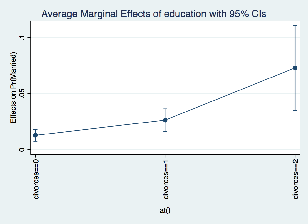
To get the effects from the previous example, I only need to take the differences between the different effects. For instance, the first interaction effect is the difference of the first and second margins, 0.026-0.013 = 0.014.
We can use margins and factor-variable notation to estimate and graph interaction effects. In the example above, I computed an interaction effect between a continuous and a discrete covariate, but I can also use margins to compute interaction effects between two continuous or two discrete covariates, as is shown in this blog article.