我们希望研究1978车辆数据中两个变量油耗和重量之间的关系。
. use auto_zh, clear
首先我们检查油耗和重量的变量描述和摘要统计数据。
. describe 油耗 重量

              storage   display    value
variable name   type    format     label      variable label
--------------------------------------------------------------------------------
油耗            float   %9.0g                 油量消耗(公升每一百公里)
重量            float   %8.0gc                重量(公斤)
. summarize 油耗

    Variable |        Obs        Mean    Std. Dev.       Min        Max
-------------+---------------------------------------------------------
        油耗 |         74     5.01928    1.279856   2.439024   8.333333
从摘要统计数据看出,变量油耗的最小值2.44,最大值8.33,极差5.89。
. summarize 重量

    Variable |        Obs        Mean    Std. Dev.       Min        Max
-------------+---------------------------------------------------------
        重量 |         74    1369.603    352.5288   798.3219   2195.385
从摘要统计数据看出,变量重量的最小值798.32,最大值2195.39,极差1397.06。
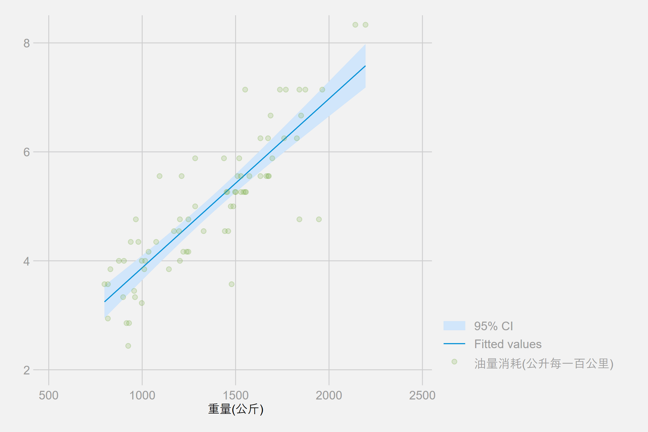
. twoway lfitci 油耗 重量 || scatter 油耗 重量, mcolor(%20) scheme(538)
我们在油耗和重量的散点图上叠加拟合值与均值的置信区间。
. regress 油耗 重量

      Source |       SS           df       MS      Number of obs   =        74
-------------+----------------------------------   F(1, 72)        =    194.71
       Model |  87.2964971         1  87.2964971   Prob > F        =    0.0000
    Residual |  32.2797637        72  .448330051   R-squared       =    0.7300
-------------+----------------------------------   Adj R-squared   =    0.7263
       Total |  119.576261        73  1.63803097   Root MSE        =    .66957

------------------------------------------------------------------------------
        油耗 |      Coef.   Std. Err.      t    P>|t|     [95% Conf. Interval]
-------------+----------------------------------------------------------------
        重量 |    .003102   .0002223    13.95   0.000     .0026589    .0035452
       _cons |   .7707669   .3142571     2.45   0.017     .1443069    1.397227
------------------------------------------------------------------------------
线性回归结果显示重量每增加一百公斤,每百公里油耗增加 0.3102公升, 可由模型解释的观察到的方差量为 73%.
. _coef_table, markdown
| 油耗 | Coef. | Std. Err. | t | P>|t| | [95% Conf. Interval] | |
|---|---|---|---|---|---|---|
| 重量 | .003102 | .0002223 | 13.95 | 0.000 | .0026589 | .0035452 |
| _cons | .7707669 | .3142571 | 2.45 | 0.017 | .1443069 | 1.397227 |
quietly regress 油耗 重量 变速比 转弯半径
estimates store 模型1
quietly regress 油耗 重量 变速比 转弯半径 国籍
estimates store  模型2
estimates table 模型1 模型2, b(%7.4f) stats(N r2_a) star
. estimates table 模型1 模型2, varlabel b(%7.4f) stats(N r2_a) star markdown
| Variable | 模型1 | 模型2 |
|---|---|---|
| 重量(公斤) | 0.0030*** | 0.0028*** |
| 变速比 | 0.1706 | -0.3367 |
| 转弯半径(米) | 0.0798 | 0.2010 |
| 国籍 | 0.8650*** | |
| Constant | -0.5814 | -0.4661 |
| N | 74 | 74 |
| r2_a | 0.7218 | 0.7637 |
legend: * p<0.05; ** p<0.01; *** p<0.001
eststo : quietly regress 油耗 重量 变速比 转弯半径
eststo : quietly regress 油耗 重量 变速比 转弯半径 国籍
esttab using esttab_ex.html, label   ///
	width(80%) nogaps                ///
	mtitles("模型1" "模型2")       ///
	title(线性回归结果)
| (1) | (2) | |
| 模型1 | 模型2 | |
| 重量(公斤) | 0.00301*** | 0.00278*** |
| (6.09) | (6.06) | |
| 变速比 | 0.171 | -0.337 |
| (0.64) | (-1.19) | |
| 转弯半径(米) | 0.0798 | 0.201 |
| (0.70) | (1.81) | |
| 国籍 | 0.865*** | |
| (3.66) | ||
| Constant | -0.581 | -0.466 |
| (-0.38) | (-0.33) | |
| Observations | 74 | 74 |
|
t statistics in parentheses
* p < 0.05, ** p < 0.01, *** p < 0.001 | ||
The community-contributed esttab is available on the Boston College Statistical Software Components (SSC) archive; see ssc install for details.